Shape optimization with CutFEM

Given these cut integrals in the interface region, we require two central ingredients:

• a way to enforce boundary conditions inside elements through integrals and not classical boundary lifting

• a stabilization technique to prevent ill-conditioning.

Nitsche’s method

Imposing Dirichlet conditions on a boundary that is not meshed explicitly requires enforcing these boundary conditions weakly via integrals. The two main approaches to enforce Dirichlet conditions weakly are Nitsche’s method [Nit71] and the Lagrange multiplier method. In this contribution, we use Nitsche’s method because it does not require an additional unknown as in the Lagrange multiplier method.

In the context of a problem solved with the finite element method on a cut mesh of \(\Omega\), the selected solution space does not inherently incorporate Dirichlet conditions (as in lifting).

Ghost penalty

A challenge arises for cut integrals, as they depend only on the physical part of elements \(\Gamma_K\) and \(\Omega_K\). Certain elements may have minimal intersection with the physical domain \(\Omega\), as depicted in Figure 11. For Nitsche’s method this can result in a penalty parameter tending to \(\infty\) (see Figure 11). Furthermore, cut elements like those shown in Figure 12 result in ill-conditioning of the system matrix.

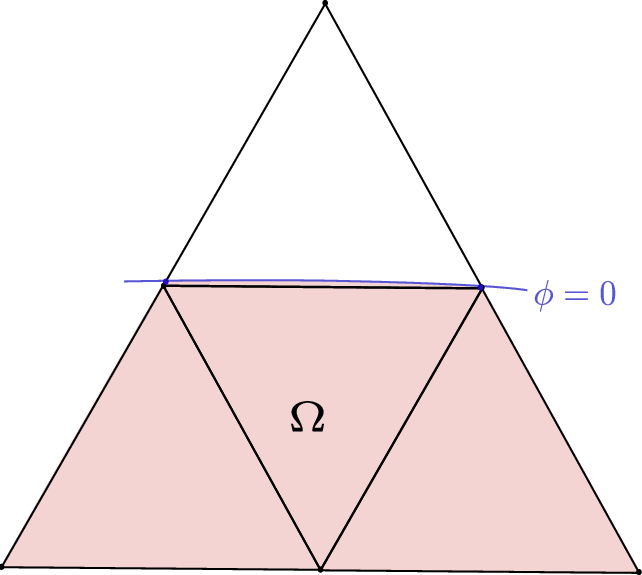
Figure 11 Example of very small intersections with the physical domain \(\Omega\) leading to a lack of stability.

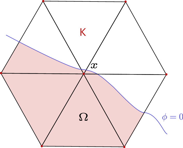
Figure 12 Example of very small intersections with the physical domain \(\Omega\) leading to an ill-conditioning.

To address these issues, one approach is to modify the formulation to depend on the active domain \(\Omega_{h}\), as illustrated by the green domain in Figure 3.This extension of the problem formulation from the physical domain (\(\Omega\)) to the active domain (\(\Omega_{h}\)) should be done accurately, ensuring that terms vanish optimally with mesh refinement and smoothness of the solution. One way to achieve such an extension is the ghost penalty stabilization method [Bur10]. The concept involves introducing a penalization term on the elements intersected by the interface \(\Gamma\). This method extends coercivity to the entire domain without compromising convergence properties.

CutFEM Weak formulation of Linear elasticity

To solve the primal problem with CutFEM we define the space of Lagrange finite elements of order \(k\) (denoted \(\mathbb{P}_{k}\)) as

(15)\[V_{h,k}:=\left\{ v\in V\left(D\right)\cap\left[C^{0}\left(D\right)\right]^{d}\mid v_{\mid K}\in\left[\mathbb{P}_{k}\left(K\right)^{d}\text{ for all }K\in\mathcal{K}_{\;h}\right]\right\}\]

and the finite element space on the active part of the mesh

(16)\[V_{h,k,\Omega}\left(\Omega_{h}\right):=V_{h,k}\mid_{\Omega_{h}}.\]

The problem formulation (4) with the finite element method on \(\mathcal{K}_{\;h}\) is: Find \(u_{h}\in V_{h,k,\Omega}\left(\Omega_{h}\right)\) such that for all \(v\in V_{h,k,\Omega}\left(\Omega_{h}\right)\)

(17)\[a\left(u_{h},v\right)+h^{2}j_{h}\left(\mathcal{F}_{h,G,\Omega};u_{h},v\right) + N_{\Gamma_{D}}\left(u_{h},v\right)=l\left(v\right)\]

with

(18)\[j_{h}\left(\mathcal{F}_{h,\Omega},u,v\right)=\sum_{F\in\mathcal{F}_{h,\Omega}}\sum_{l=1}^{k}\gamma_{a}h^{2l-1}\left(\left[\partial_{n_{F}}^{l}u\right],\left[\partial_{n_{F}}^{l}v\right]\right)_{L^{2}\left(F\right)}\text{ where }\gamma_{a}>0\]

Here,

(19)\[\left[v\right]=v\mid_{K_{+}}-v\mid_{K_{-}}\]

denotes the jump across facet \(F\) between element \(K_{+}\) and \(K_{-}\) and \(n_F\) is the normal to facet \(F\). The term \(j_h\) is called ghost penalty stabilization and guarantees well conditioned system matrices. The term \(N_{\Gamma_D}\) are the terms of Nitsche’s method to impose Dirichlet conditions on \(\Gamma_{D}\) defined as

(20)\[\begin{split}\begin{split} N_{\Gamma_{D}}\left(u,v\right)=&\left(\sigma(u)\cdot n,v\right)_{L^{2}\left(\Gamma_{D}\right)}-\left(u,\sigma\left(v\right)\cdot n\right)_{L^{2}\left(\Gamma_{D}\right)}\\ &+\frac{\gamma_{D}}{h}\left[2\mu\left(u,v\right)_{L^{2}\left(\Gamma_{D}\right)}+\lambda\left(u\cdot n,v\cdot n\right)_{L^{2}\left(\Gamma_{D}\right)}\right], \end{split}\end{split}\]

where \(\gamma_{D}>0\) is a penalty parameter independent of the mesh size \(h\).

Advection

To transport the domain using the level-set method we have to solve the transport equation (6). To stabilize this equation, we introduce a stabilization parameter \(\gamma_{\text{Adv}}>0\), and use the inner stabilization proposed in [BEH+18]:

(21)\[\left(\partial_{t}\phi,v\right)_{L^{2}\left(D\right)}+\left(v_{\text{reg}}\left|\nabla\phi\right|, v\right)_{L^{2}\left(D\right)}+\gamma_{\text{Adv}}\sum_{F\in\mathcal{F}_{h,\Omega}}h^{2}\left(\left[\partial_{n_{F}}\phi\right],\left[\partial_{n_{F}}v\right]\right)_{L^{2}\left(F\right)}=0.\]