Compliance minimization

Minimizing the compliance of a structure is a classic problem that has been the subject of numerous studies.

Problem definition

We seek the optimal shape, \(\widetilde{\Omega}\subset D\), that minimizes the compliance of the structure for a linear elastic material subject to Dirichlet and Neumann boundary conditions. We impose a target area on the structure, which results in the addition of an equality constraint. The optimization problem is defined as

\[\begin{split}\begin{align}\begin{cases} \underset{\Omega\in\mathcal{O}}{\min}J(\Omega) & \!\!\!\!=\underset{\Omega\in\mathcal{O}}{\min}\int_{\Omega}(\mu\varepsilon(u):\varepsilon(u)+\frac{\lambda}{2}\nabla\cdot u\nabla\cdot u)\text{ }dx\\ C(\Omega) & \!\!\!\!=0\\ a\left(u,v\right) & \!\!\!\!=l\left(v\right) \end{cases}\end{align}\end{split}\]

u is the displacement field solution to PDE equation and the constraint over the area is defined as:

\[C(\Omega)=\int_{\Omega}dx - \overline{V}\]

with \(\overline{V}\) the target volume.

Shape derivative

Using the Céa method the shape derivative of the compliance minimization problem is defined as :

\[\begin{align} J'(\Omega)(\theta) &= -\int_{\partial\Omega}\theta\cdot n[ \mu\varepsilon(u_{\Omega}):\varepsilon(u_{\Omega})+\frac{\lambda}{2}(\nabla\cdot u_{\Omega})(\nabla\cdot u_{\Omega})]\text{ }ds \end{align}\]

where \(n\) is the unit normal.

To account for the constraint in the optimization, the ALM (see Augmented lagrangian Method ) is used. First, we define the modified cost function as:

\[\begin{align} \mathcal{J}(\Omega) &= J(\Omega) +\alpha C(\Omega)+\frac{\beta}{2} C^{2}(\Omega). \end{align}\]

Then, we calculate the shape derivative of this new function. We obtain the following shape derivative:

\[\begin{align} \mathcal{J}'(\Omega)(\theta) &= J'(\Omega)(\theta) +\alpha C'(\Omega)(\theta) +\beta C(\Omega)C'(\Omega)(\theta). \end{align}\]

Using the shape optimization algorithm, the descent direction is directly defined as:

\[v(u_{\Omega}) = 2\mu\varepsilon(u_{\Omega}):\varepsilon(u_{\Omega})+\lambda(\nabla\cdot u_{\Omega})(\nabla\cdot u_{\Omega}) + \alpha+\beta C(\Omega).\]

Algorithm

\[\begin{split}\begin{array}{l} \textbf{BEGIN} \\ \quad u_{h} \gets \text{Resolution of Primal problem (elasticity linear): } a\left(u,v\right)=l\left(v\right)\\ \quad \text{WHILE } \left\Vert J\left(\Omega_{n+1}\right)-J\left(\Omega_{n}\right)\right\Vert <tol \text{:} \\ \quad \quad n \gets n+1 \\ \quad \quad \lambda_{ALM}^{n},\mu_{ALM}^{n} \gets \text{ Update ALM parameters}\\ \quad \quad v \gets \text{Explicit calculation of the velocity, defined on }\Gamma \\ \quad \quad v_{ext} \gets \text{Extension of the velocity in } D\\ \quad \quad v_{\text{reg}} \gets \text{Normalization of the velocity} \\ \quad \quad \text{WHILE adv_NAN}\neq1 \\ \quad \quad \quad \phi_{\text{temp}} \gets \text{Advection }\\ \quad \quad \quad \phi_{\text{temp}} \gets \text{Reinitialization}\\ \quad \quad \quad u_{h} \gets \text{Resolution of Primal problem (elasticity linear): } a\left(u,v\right)=l\left(v\right)\\ \quad \quad \quad \text{dt, } j_{\text{max}} \text{, adv_NAN} \gets \text{Update parameters}\\ \quad \quad \phi \gets \phi_{temp}\\ \textbf{END}\\ \end{array}\end{split}\]

Application

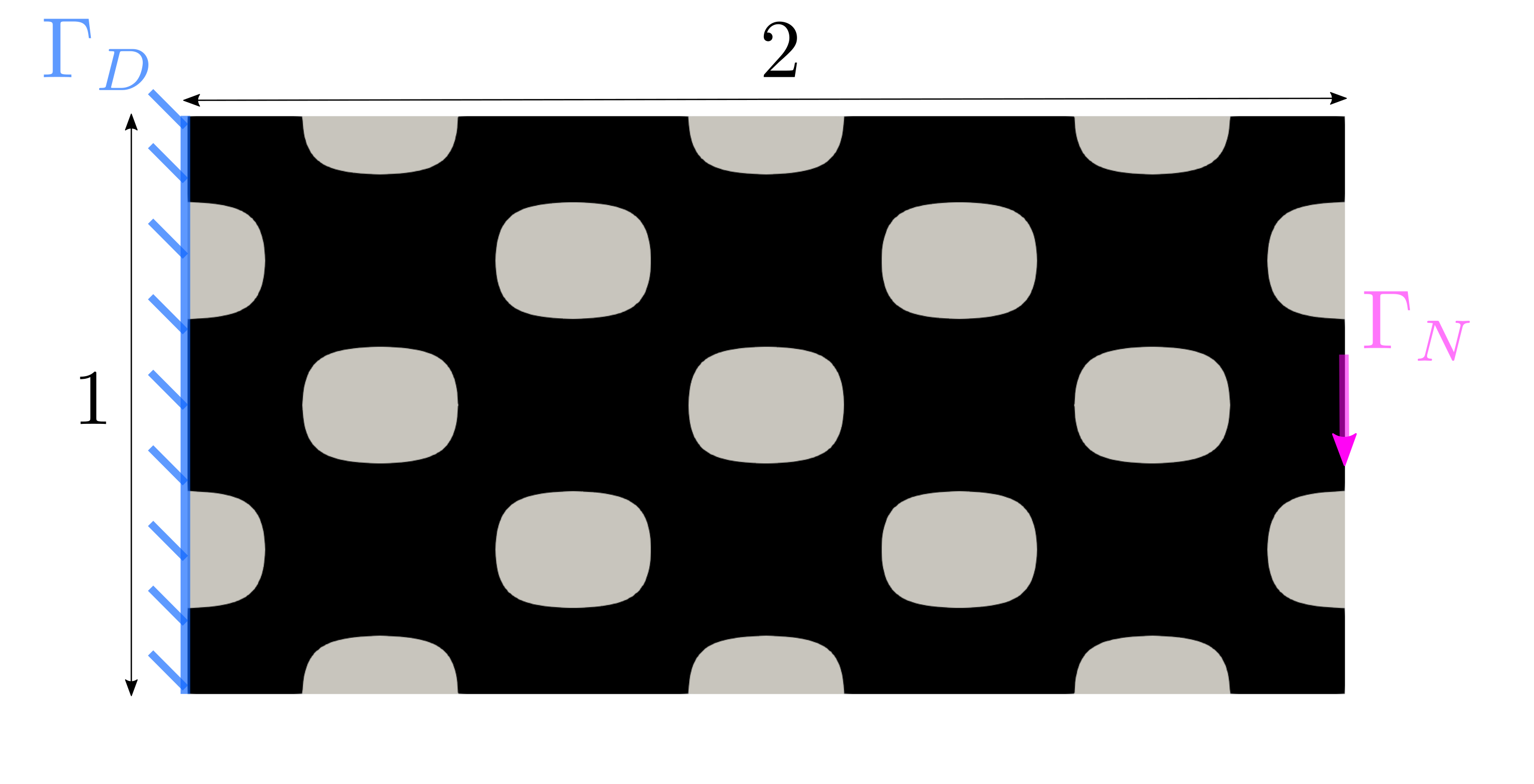
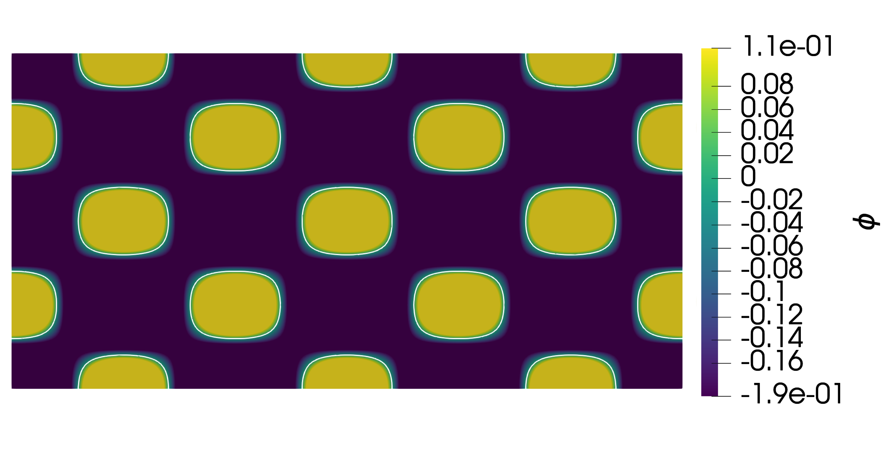
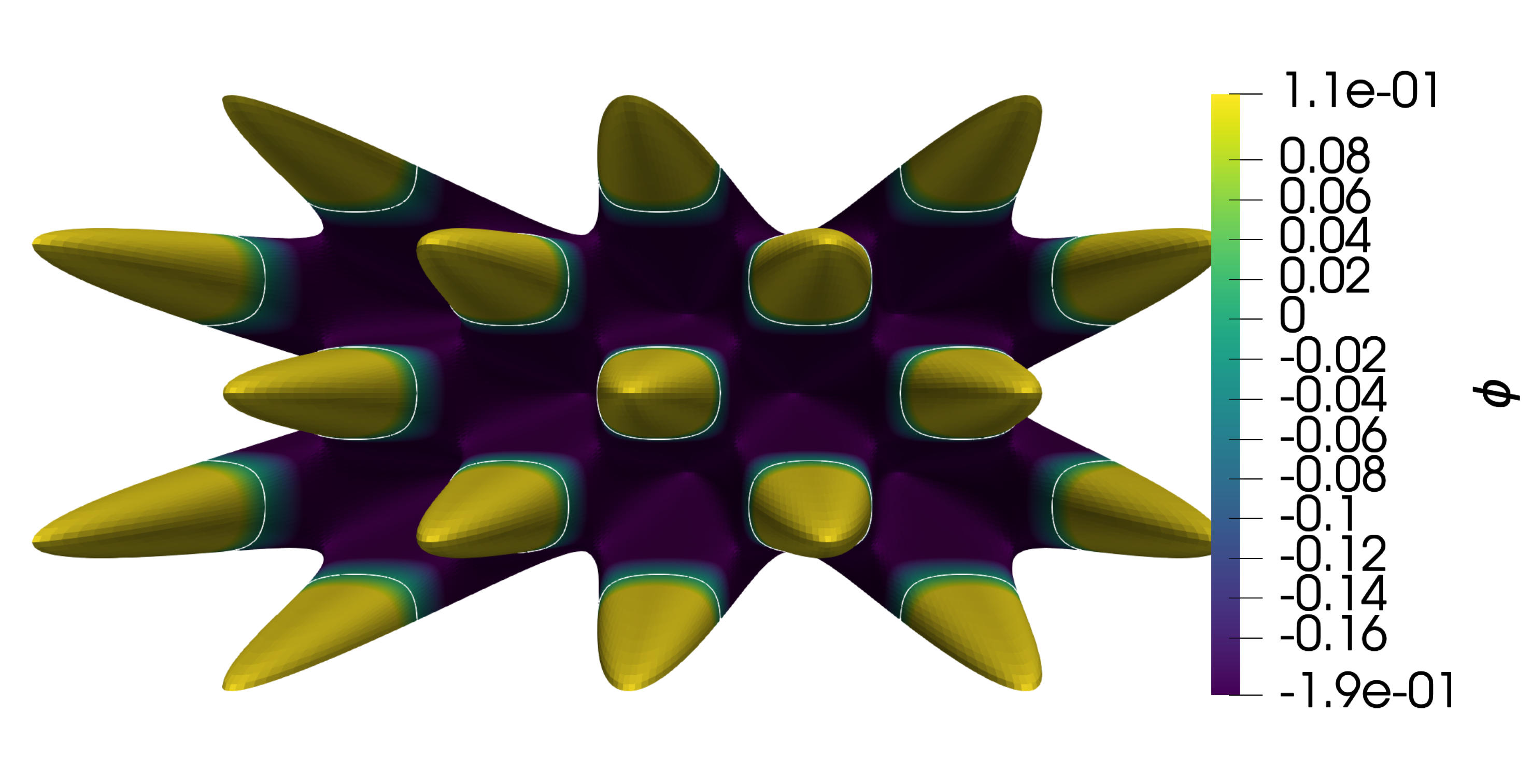
We study the case of an embedded steel beam of \(1\text{m}\times 2\text{m}\) subjected to a uniformly distributed tensile load at \(\pm 0.5\) m such that \(g=-0.1 e_{y}\) GPa. The numerical values used as parameters in the mechanical model are detailed in the Table 1. The domain \(\Omega\) included in \(D\) is initialized as shown in Figure 13, and it is discretized with a \(100\times200\) finite element mesh. The problem is solved with a target area of \(1.2 \text{ m}^{2}\) and an initial area of \(1.64m^{2}\). The optimal shape obtained is shown in CutFEM solution with CutFEM method and in Ersatz solution for Ersatz method.

Figure 13 Initialization of \(\Omega\subset\text{D}\)

Figure 14 Initialization of the mesh.

Table 1 Mechanical parameters

Parameter	Value	Unity
E (Young Modulus)	210	GPa
\(\nu\)	0.33
Strength	0.1	GPa

Initialization of all parameters

The first step is to instantiate the Parameter object and then initialize all of its attributes using the provided data file named “param_compliance.txt”.

parameters = Parameters("compliance")
name = "param_compliance.txt"
parameters.set__paramFolder(name)

Mesh Generation

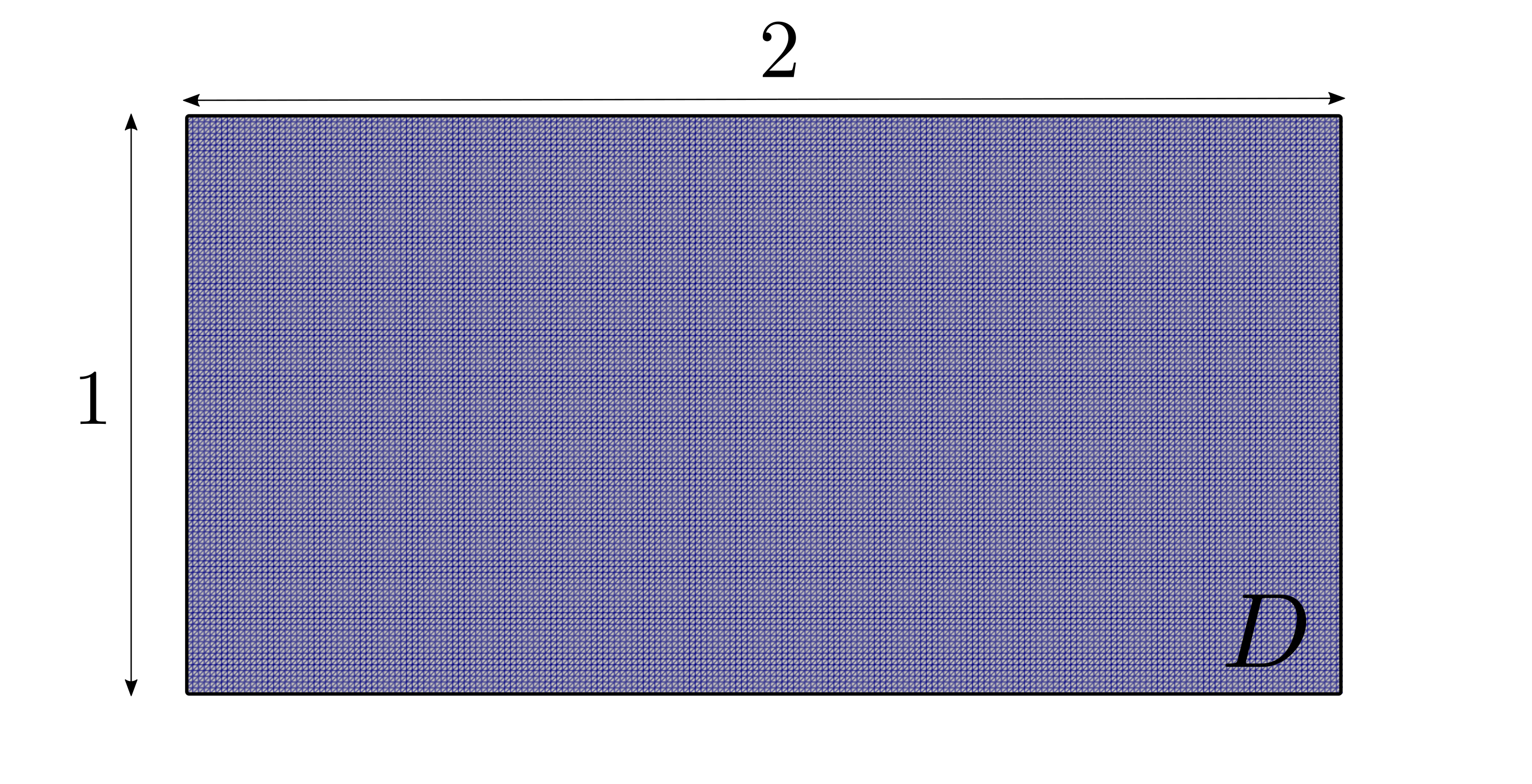
Then to generate the rectangular mesh seen in Figure 14 the function create_mesh.create_mesh_2D() is called.

from create_mesh import *

msh = create_mesh_2D(parameters.lx, parameters.ly, int(parameters.lx/parameters.h),int(parameters.ly/parameters.h))

Initialization of the spaces

Next, we generate the spaces for all the functions that will be used.

V = fem.functionspace(msh, ("Lagrange", 1, (msh.geometry.dim, )))
V_vm = fem.functionspace(msh, ("Lagrange", 2, (msh.geometry.dim, )))
V_ls = fem.functionspace(msh, ("Lagrange", 1))
Q = fem.functionspace(msh, ("DG", 0))
V_DG = fem.functionspace(msh, ("DG", 0, (msh.geometry.dim, )))

# Initialization of the spacial coordinate
x = ufl.SpatialCoordinate(msh)

Initialization of the level set

To initialize the level set function, we use the module geometry_initialization() and the function : geometry_initialization.level_set(). In this module, we define all the desired initializations for the level set function and adjust the call based on the desired configuration.

import geometry_initialization

ls_func_ufl = geometry_initialization.level_set(x,parameters)
ls_func_expr = fem.Expression(ls_func_ufl, V_ls.element.interpolation_points())
ls_func = Function(V_ls)
ls_func.interpolate(ls_func_expr)

Figure 15 Initialization of the level set.

Figure 16 Initialization of the level set warped.

Initialization of the boundary conditions

We define the Dirichlet conditions for the linear elasticity problem, denoted \(\Gamma_{D}\) in Figure 13.

import numpy as np
from dolfinx import fem, mesh

fdim = msh.topology.dim - 1 # facet dimension

def clamped_boundary_cantilever(x):
        return np.isclose(x[0], 0)

boundary_facets = mesh.locate_entities_boundary(msh, fdim,clamped_boundary_cantilever)
u_D = np.array([0,0], dtype=ScalarType)

bc = fem.dirichletbc(u_D, fem.locate_dofs_topological(V, fdim, boundary_facets), V)

We define the Neumann conditions for the linear elasticity problem, denoted \(\Gamma_{N}\) in Figure 13. Then, we define Dirichlet boundary condition for the velocity field.

import numpy as np
from dolfinx.mesh import meshtags


def load_marker(x):
        return np.logical_and(np.isclose(x[0],parameters.lx),np.logical_and(x[1]<(0.55),x[1]>(0.45)))

# Boundary condition for the velocity field.
boundary_dofs = fem.locate_dofs_geometrical(V_ls, load_marker)
bc_velocity = fem.dirichletbc(ScalarType(0.), boundary_dofs, V_ls)

# Neumann boundary condition for the primal problem.
facet_indices, facet_markers = [], []
facets = mesh.locate_entities(msh, fdim, load_marker)
facet_indices.append(facets)
facet_markers.append(np.full_like(facets, 2))

facet_indices = np.hstack(facet_indices).astype(np.int32)
facet_markers = np.hstack(facet_markers).astype(np.int32)
sorted_facets = np.argsort(facet_indices)
facet_tag = meshtags(msh, fdim, facet_indices[sorted_facets], facet_markers[sorted_facets])
ds = ufl.Measure("ds", domain=msh, subdomain_data=facet_tag)

Instantiation of the objects

We instantiate the objects of the following classes:

• Reinitialization (levelSet_tool.Reinitialization()),

• ErsatzMethod (ersatz_method.ErsatzMethod()),

• CutFemMethod (cutfem_method.CutFemMethod()).

Then, we initialize the coefficients of Lamé with the function mechanics_tool.lame_compute().

Reinitialization = Reinitialization(ls_func, V_ls=V_ls, l=parameters.l_reinit)

ErsatzMethod = ErsatzMethod(ls_func,V_ls, V, ds = ds, bc = bc, parameters = parameters, shift = shift)

CutFemMethod = CutFemMethod(ls_func,V_ls, V, ds = ds, bc = bc, parameters = parameters, shift = shift)

lame_mu,lame_lambda = mechanics_tool.lame_compute(parameters.young_modulus,parameters.poisson)

Instantiation of Problem class

We instantiate the problem class. Here, we aim to minimize the compliance, so the problem is of the Compliance_Problem class. Defining the problem object then allows for automating the call of functions to calculate the cost, its integrand, the integrand of the cost’s derivative, the constraint value, the integrand of the constraint, the integrand of the derivative of the constraint, and the dual operator if necessary. See problem.Compliance_Problem() for clarification.

problem_topo = problem.Compliance_Problem()

Resolution of linear elasticity

Our code offers two methods for the optimization problem: the ersatz material method and the CutFEM method. Here, we demonstrate the implementation of both methods for solving the linear elasticity problem.

if parameters.cutFEM == 1:
        CutFemMethod.set_measure_dxq(ls_func)
        uh = CutFemMethod.primal_problem(ls_func_temp,parameters)

        measure = CutFemMethod.dxq
else:
        xsi = ErsatzMethod.heaviside(ls_func)
        uh = ErsatzMethod.primal_problem(ls_func_temp, parameters)

        measure = ufl.dx

cost = problem_topo.cost(uh,ph,lame_mu,lame_lambda,measure,parameters)

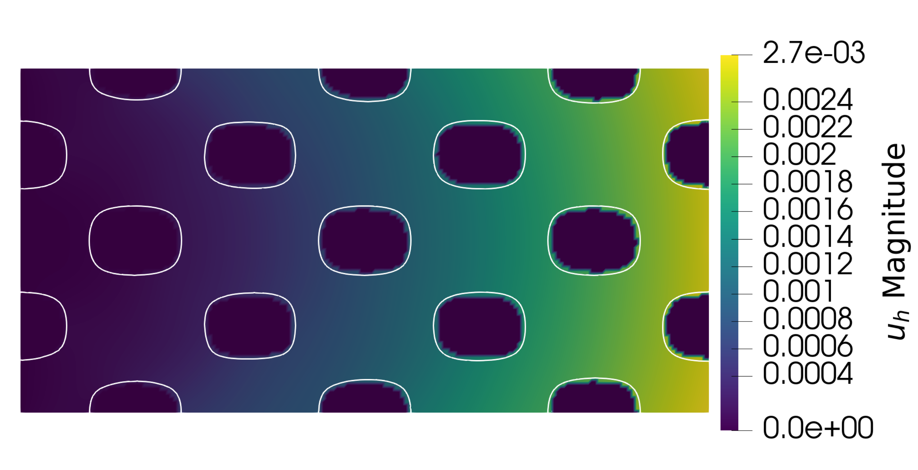
Figure 17 Displacement field of the first iteration with CutFEM.

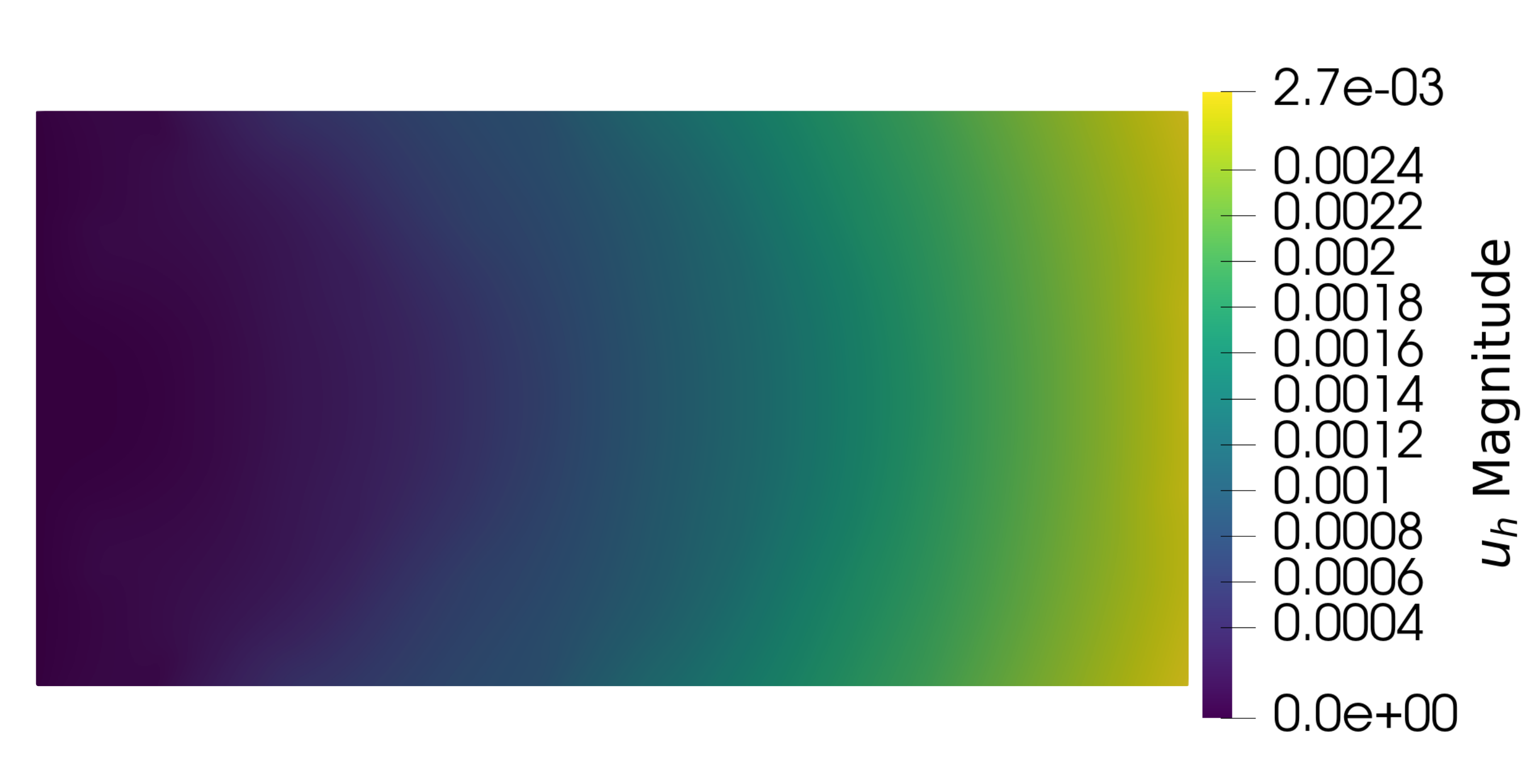
Figure 18 Displacement field of the first iteration with Ersatz method.

Note

To remind, the differences CutFEM and Ersatz primal problem are defined in (17) and in (5).

Note

The heaviside function is needed for the ersatz method. The definition is given by (14) and we choose \(\varepsilon=0.001\).

Shape derivative computation

shape_derivative = problem_topo.shape_derivative_integrand(uh,ph,lame_mu,lame_lambda,parameters,measure)

rest_constraint = problem_topo.constraint(uh,lame_mu,lame_lambda,parameters,measure,(1-parameters.cutFEM)*xsi)

shape_derivative_integrand_constraint = problem_topo.shape_derivative_integrand_constraint(uh,ph,lame_mu,lame_lambda,parameters,measure)

Note

For the compliance minimization the dual solution is automatically initialized as zero function.

Update ALM parameters

To update the Augmented Lagrangian parameters we call the almMethod.maj_param_constraint_optim():

almMethod.maj_param_constraint_optim(parameters,rest_constraint)

Note

To simplify, the penalization method can also be used by simply initializing parameters.ALM to 0. The penalization value must be chosen very carefully, depending on the problem.

Compute the descent direction

To compute the advection velocity, we first call on of this two functions :

• cutfem_method.CutFemMethod.descent_direction()

• ersatz_method.ErsatzMethod.descent_direction()

depending on the chosen method.

Next, we normalize the solution field using an adaptation of the H1 norm by calling the function cutfem_method.CutFemMethod.velocity_normalization() . Finally, we compute the maximum of the velocity field to determine a time step for advection that satisfies the CFL condition.

velocity_field = problem_topo.descent_direction(CutFemMethod.level_set,msh,parameters,bc_velocity,V_ls,\
                                    V_DG,rest_constraint,shape_derivative_integrand_constraint,shape_derivative)
velocity_field = CutFemMethod.velocity_normalization(velocity_field,parameters.alpha_reg_velocity)

velocity_expr = fem.Expression(velocity_field, V_ls.element.interpolation_points())
velocity = fem.Function(V_ls)
velocity.interpolate(velocity_expr)

max_velocity = comm.allreduce(np.max(np.abs(velocity.x.array[:])),op=MPI.MAX)

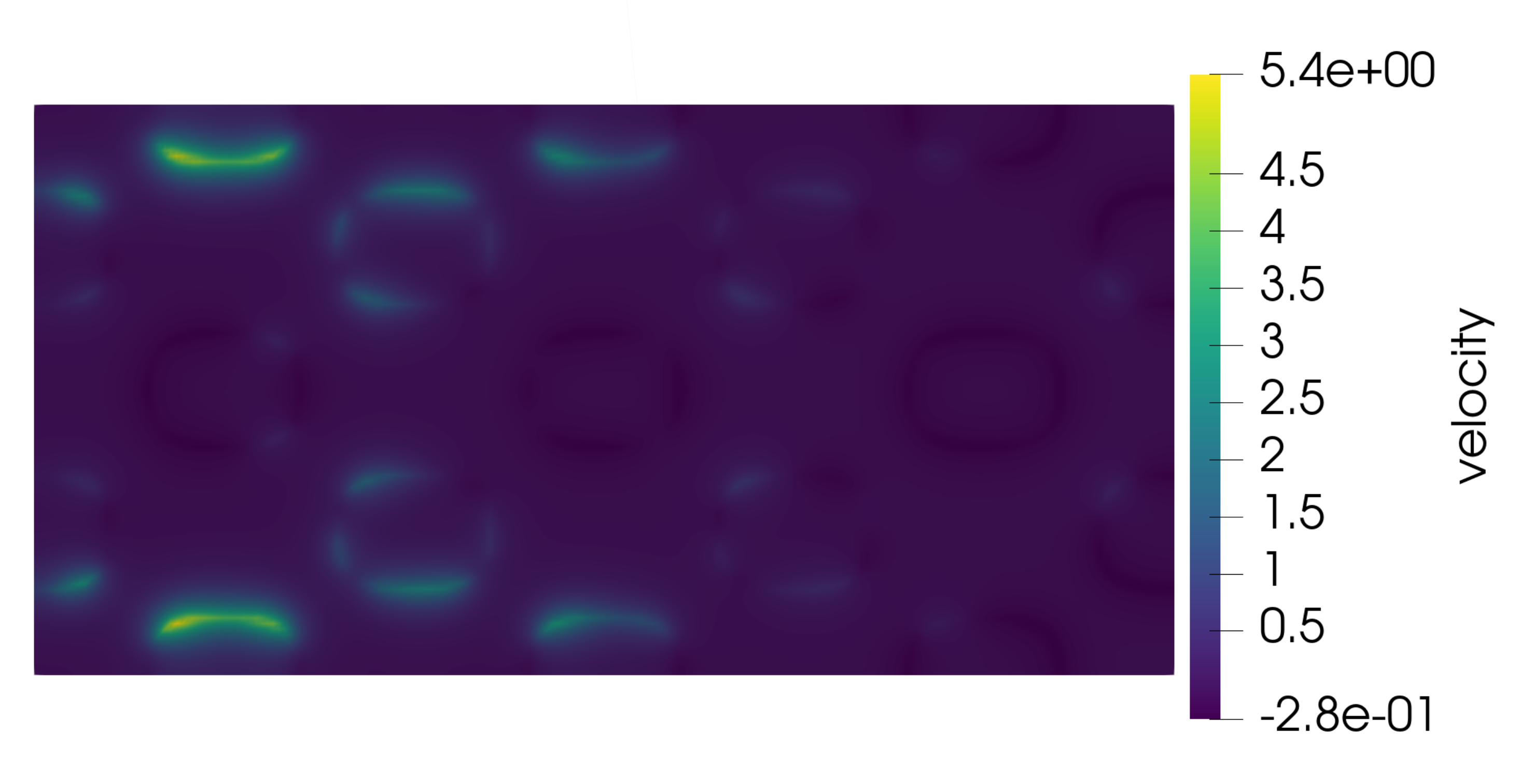
Figure 19 Velocity field of the first iteration.

Advection of the level set function

To advect the level set in the computed descent direction, we call the function cutfem_method.CutFemMethod.cut_fem_adv(). To optimize our code, we first call opti_tool.adapt_c_HJ(), which optimizes the choice of the parameter c when computing the advection time step. This function uses the evolution of the convergence criterion to gradually decrease the value of c. Then, the function opti_tool.adapt_dt() is called to adjust the advection time step.

c_param_HJ = opti_tool.adapt_c_HJ(c_param_HJ,crit,parameters.tol_cost_func,lagrangian)

parameters.dt  =  opti_tool.adapt_dt(lagrangian_cost,lagrangian_cost_previous,max_velocity,parameters,c_param_HJ)

ls_func_temp = CutFemMethod.cut_fem_adv(ls_func_temp,(1/adv_bool)*parameters.dt, velocity_field)

Reinitialization of the level set

To reinitialize the level set using the P.C. method after setting the number of frequency for the reinitialization to parameters.step_reinit we call the method levelSet_tool.Reinitialization.reinitializationPC()

if ((j%parameters.freq_reinit)==0):
        ls_func_temp, temp_func = Reinitialization.reinitializationPC(ls_func_temp,parameters.step_reinit)

Note

The frequency of the reinitialization is the number of iterations of optimization problem we want to do after reinitialized the level set function. For this exemple we set it to \(1\).

Figure 20 Initialization of the level set.

Figure 21 Reinitialized level set function.

Figure 22 Initialization of the level set.

Figure 23 Reinitialized level set function.

Update all the parameters

parameters.dt, adv_bool = opti_tool.catch_NAN(cost,lagrangian_cost,rest_constraint,parameters.dt,adv_bool)

if adv_bool<2:
        parameters.j_max = opti_tool.vm_adapta_HJ(lagrangian_cost,lagrangian_cost_previous,parameters.j_max,parameters.dt,parameters)
else:
        parameters.j_max = 1

CutFEM solution

The results of the optimization with the CutFEM method, obtained after a fixed number of iterations set to 300, are provided below. The geometry of the domain obtained corresponds to the usual results found in the literature. It is observed that the constraint imposed on the volume is well satisfied.

Ersatz solution

The results of the optimization with the fictitious material method, obtained after a fixed number of iterations set to 300, are provided below. The geometry of the domain is very similar to the previous one, obtained with CutFEM. It is observed that the constraint imposed on the volume is also well satisfied.